Exercise 1: Partitioning & Parallel Query Processing

Recall the products database from DSCB that consists of 4 relational instances with the following schemas

Product(maker, model, type) 
Laptop(model, speed, ram, hd,screen, price)
PC(model, speed, ram, hd, price) 
Printer(model, color, type, price)

The Product relation gives the manufacturer, model number and type ( PC, laptop, or printer ) of various products. We assume for convenience that model numbers are unique over all manufacturers and product types; that assumption is not realistic, and a real database would include a code for the manufacturer as part of the model number. The PC relation gives for each model number that is a PC the speed ( of the processor, in gigahertz ), the amount of RAM ( in megabytes ), the size of the hard disk ( in gigabytes ), and the price. The Laptop relation is similar, except that the screen size ( in inches ) is also included. The Printer relation records for each printer model whether the printer produces color output ( true, if so ), the process type ( laser or ink - jet, typically ), and the price.

Assume a shared-nothing parallel database system on 4 nodes. Further assume that query results need to be transferred back to the node where the query originates. Consider the following query on the Laptop relation

SELECT model
FROM Laptop
WHERE ram>2048

a) Draw the task scheduling graph (like a Gantt chart) assuming horizonal partitioning using ranges on the ram attribute.

b) Draw the task scheduling graph (like a Gantt chart) assuming horizonal partitioning using hashing on the model attribute.

c) Draw the task scheduling graph (like a Gantt chart) assuming vertical partitioning on all attributes.

d) Discuss implications of partitioning on communication cost, load balancing, latency, etc.

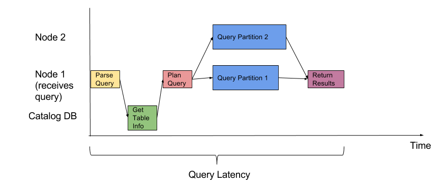
Here’s an example of a task scheduling graph: